Drawing Pictures with Epicycles

Introduction

Perhaps, while surfing the web, you’ve come across an animation that looked like this:

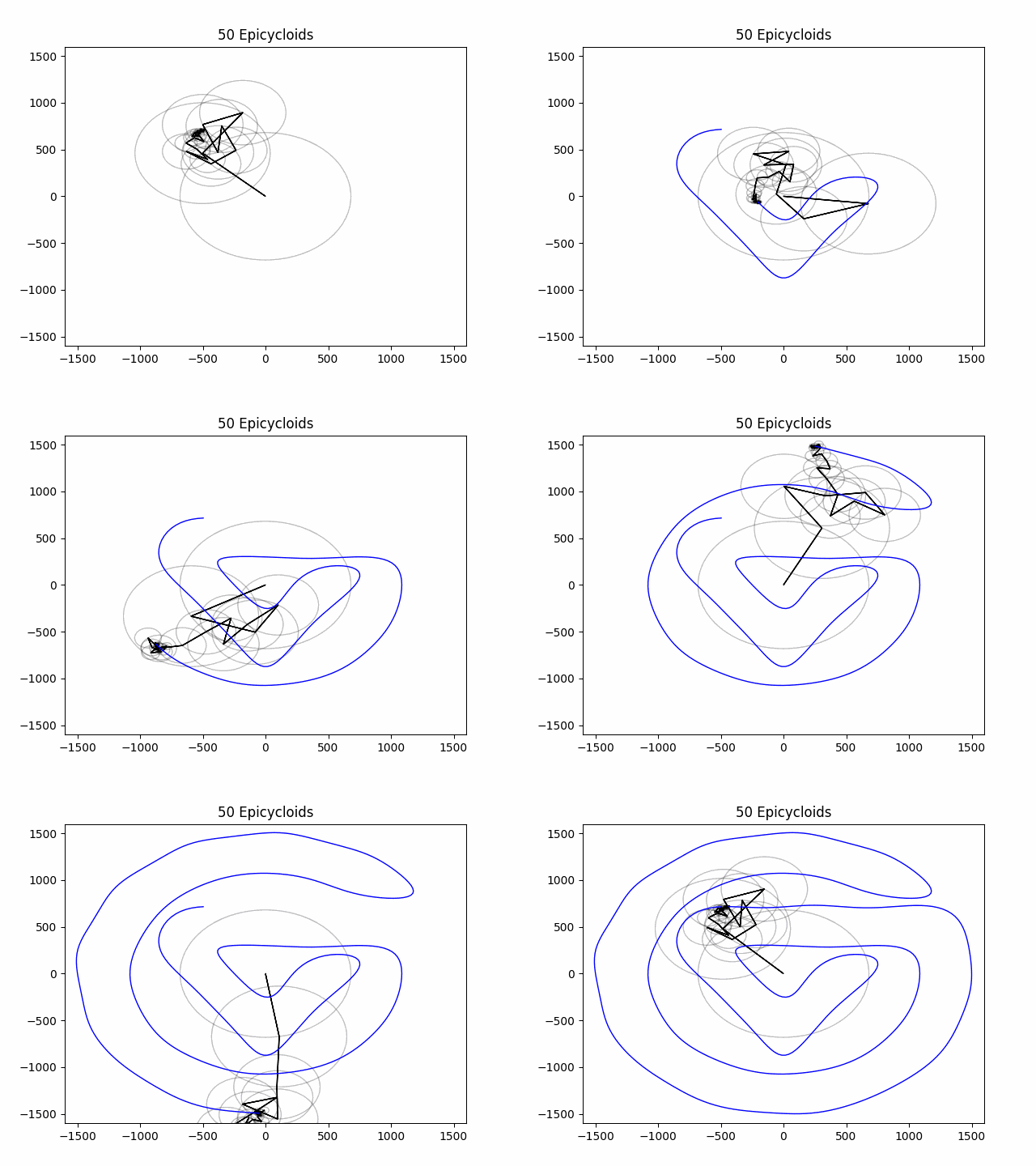
Dozens of circles rotating around each other, with the very tip of the line they create tracing out a drawing. This fascinated me, and I had to know how this is done. As it turns out, there is a great deal of mathematics behind such a simple drawing. I wanted to learn how to make my own animations like this, and I’m going to show you how these animations work and how I made my own in python.

The Mathematics Behind the Animations

Before we begin to discuss how these animations are created, there is a decent amount of mathematics we have to discuss. Don’t worry, we are going to explain everything you’ll need to know in this section.

Complex Numbers

You have probably encountered complex numbers in one of your high school math classes. As a quick refresher, we can define a new number called $i$, where $i^2 = -1$, implying that $i = \sqrt{-1}$. We can then define a complex number $z$ to have the form $z = x + yi$, where $x$ and $y$ are the real and imaginary parts of $z$, respectively.

If we let $z = x + yi$, then we denote the real and imaginary parts of $z$ as \(\textbf{Re}(z) = x, \\ \textbf{Im}(z) = y.\)

The Modulus and Argument of $z$

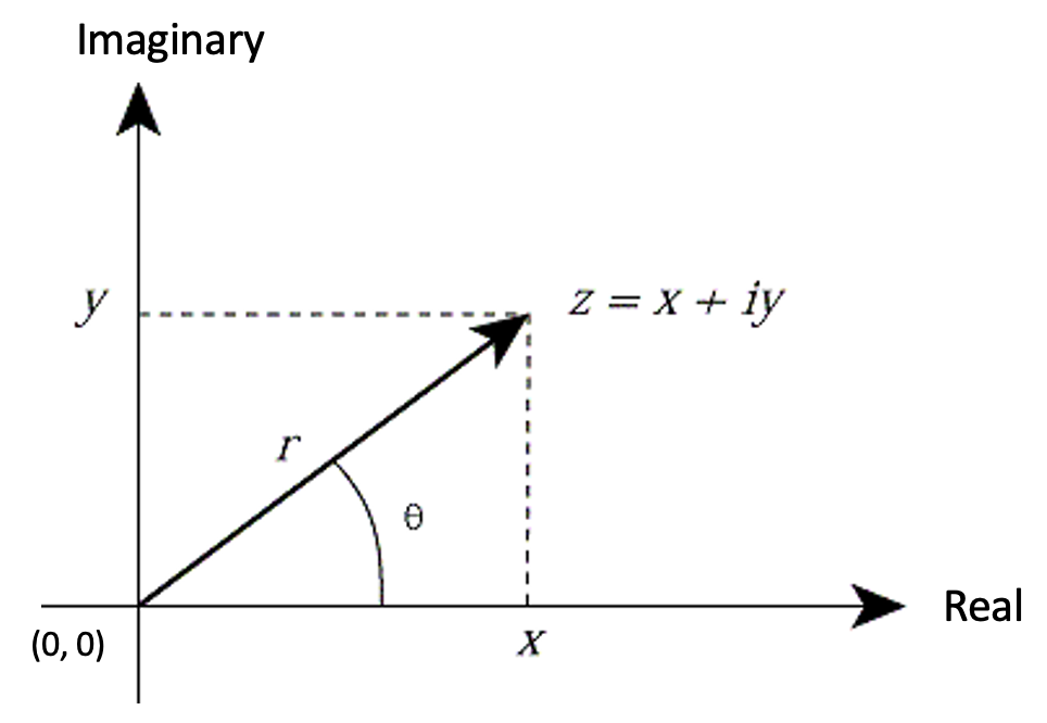
We can graph a complex number on something called the complex plane. This plane is the same as the 2D graph, except the $y$-axis is multiplied by $i$. We call this new axis the imaginary axis.

We can think of our complex number $z$ as a line, drawn from the origin to the point $(x, y)$. This line has some important properties, namely the modulus and argument of $z$.

The modulus of $z$, denoted as |$z$| , is the length of the line formed by plotting our point on the complex plane. In the above image, |$z$| $= r$. If $z = x + yi$, then we can use the Pythagorean Theorem to see that

\[|z|= \sqrt{x^2+y^2}\]

The argument of $z$, denoted as $\textbf{Arg}(z)$, is the angle formed by the line and the positive $x$-axis. In the above image, $\textbf{Arg}(z) = \theta$. By convention, we say that $0 \leq \textbf{Arg}(z) < 2\pi$, since any argument outside of this range could be represented as an argument inside of this range. If $z = x + yi$, then we see that \(\textbf{Arg}(z) = \arctan (\frac{y}{x}).\)

Epicycles

Let’s break down the word epicycle. The prefix, epi- comes from Greek, meaning upon, at, or on top of. The suffix -cycle also comes from Greek, meaning circle. We can think about epicycles as circles on top of circles, and in our case we can think of circles rotating over other rotating circles.

For example, consider the rotation of the Earth around the Sun, pictured below.

INSERT GIF LATER

Notice how the Earth rotates around the sun in a circle, as shown by the line traced behind it. We can consider the Moon rotatating around the Earth as well, as is shown below.

INSERT GIF LATER

Notice that the Moon’s orbit is much faster than the sun, but both are circular. We can think of these orbits as epicycles, and define some of their key characteristics.

We call the speed of which the circle spins it’s frequency of the epicycle, and the angle that the point along the circumference begins it’s orbit the phase of the epicycle.

The Discrete Fourier Transform

The DFT is one of the most powerful tools in signal processing, used to analyze the frequency of a periodic function through equally-spaced samples. However, we will be using the DFT for something known as trigonometric interpolation.

What is Trigonometric Interpolation?

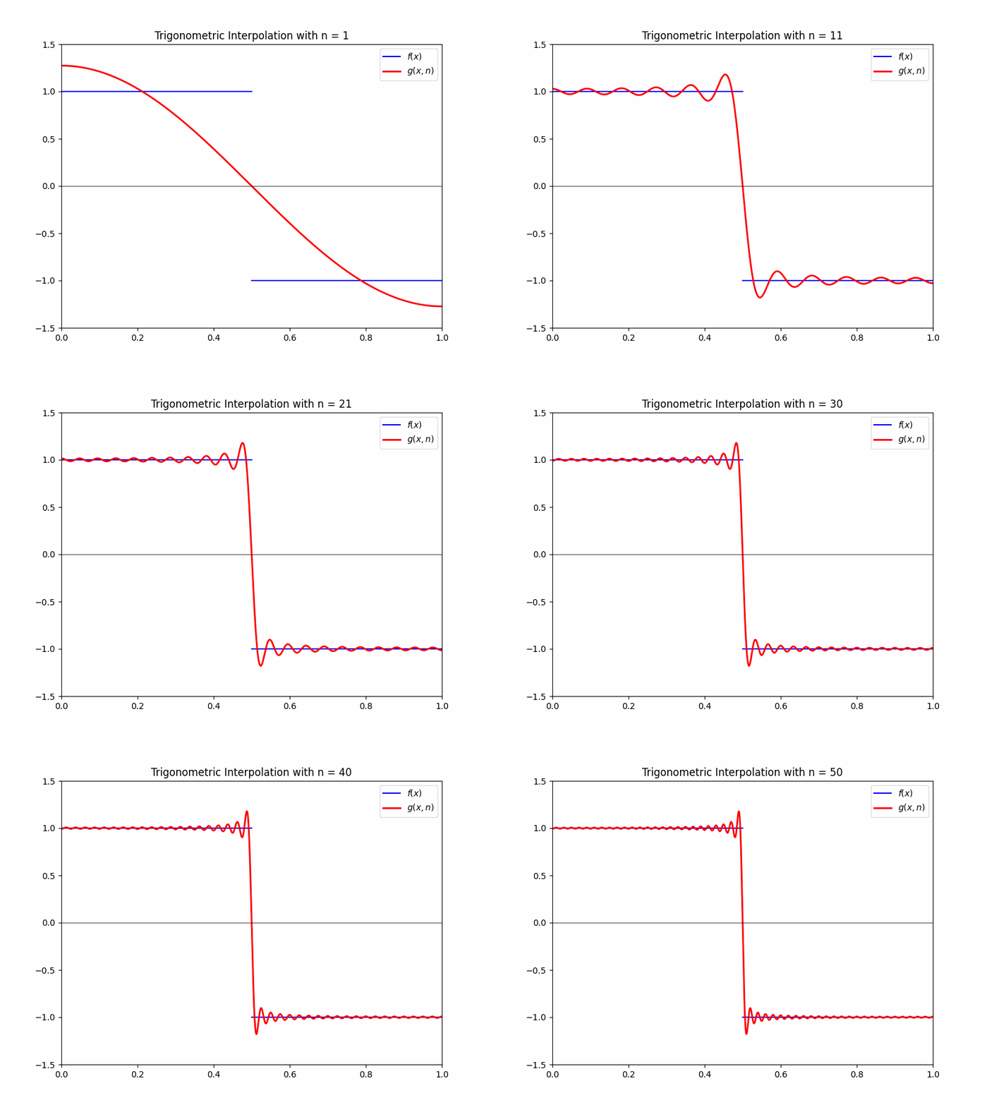
Trigonometric interpolation is the process of approximating a function as a sum of various sin or cosine functions. For example, consider the function

\[f(x) = \begin{cases} 1 & \text{if} & x < 0.5 \\ 0 & \text{if} & x = 0.5 \\ -1 & \text{if} & x > 0.5 \end{cases}\]

which is shown in the graph below.

We can approximate this function with the DFT as a summation of cosine waves. Without getting too into the number-crunching, we end up with the approximation

\[g(x,n) = \frac{4}{\pi} \sum_{i=1}^n \left(\frac{\cos{(2i-1) \pi x}}{2i-1}\right)(-1)^{i+1}\]

where $n$ is a positive integer. This function has the property that, as $n$ gets large, $g(x,n)$ approaches $f(x)$. That is,

\[\lim_{n \rightarrow \infty}g(x, n) = f(x).\]

This is shown in the following gif:

The Formula for the DFT

The Discrete Fourier Transform (DFT) is fairly complex (pun intended). I’m going to define the formula, and then talk through it with you. The DFT is defined as

\[X_k = \frac{1}{N} \sum_{n=0}^{N-1} x_n \left[ \cos{\left( \frac{2 \pi k n}{N}\right)} - i \sin{\left( \frac{2 \pi k n}{N}\right)}\right].\]

Basically, the DFT turns a sequence of $N$ complex numbers

\[x := x_0, x_1, \dots, x_{N-1}\]

into a different sequence of complex numbers,

\[X := X_0, X_1, \dots, X_{N-1}.\]

In our context, if we let $f(x)$ be the function we want to approximate, then

• $N =$ number of samples we have from $f$
• $n =$ the index of the sample from our sequence $(0, 1, \dots, N-1)$
• $x_n =$ a complex representation of our function at time $n$, in the form $x + f(x)i$
• $k =$ the current frequency we are considering $(0\text{ Hz}, 1\text{ Hz}, \dots, N-1\text{ Hz})$
• $X_k =$ amount of frequency $k$ in $f$ (amplitude and phase represented as a complex number)

Okay… how does this help us draw?

The DFT shows us the frequencies that make up a function, as shown below. If we can turn these frequencies into epicycles somehow, maybe we would be able to chain them together, let them rotate, and they would approximately draw out our original function!

We can treat the coordinates of the periodic image that we would like to trace out as complex numbers, where the point $(x,y)$ turns into the complex number $x+iy$ Then we can use the DFT to convert this discrete set of points into a new sequence of complex points. This new sequence tells us the frequencies and phases needed for each epicycle in order to approximately trace out the given image!

We can think of this as a two dimensional trigonemetric interpolation, which is why it is important that the given sequence of coordinates needs to be periodic. This ensures that the gif will loop correctly, without ending in a different spot than it began.

Python Implementation

Now that we have a grasp on the underlying mathematics of drawing with epicycles, let’s implement this programatically!

I will be using Python to generate these gifs, along with several python packages such as matplotlib and numpy.

Load our Coordinates

First, we need an image to draw. For the animation to work, we need a collection of points on the complex plane that trace out the edge of our shape. I used an SVG found on GVSU’s Identity Website, and plugged it into a website called coördinator to extract the $x$ and $y$ coordinates.

These coordinates were saved to my GVSU Google Drive, and are accessed below.

import csv
# Read our CSV file and extract the coordinates
x_coords = []
y_coords = []
with open('/content/drive/MyDrive/GV-Logo-Coords.csv', mode='r') as file:
    csv_reader = csv.DictReader(file)
    for row in csv_reader:
        x_coords.append(float(row['x']))
        y_coords.append(float(row['y']))

To keep things simple, lets normalize these coordinates to the range $[-1, 1]$.

# Function to normalize coordinates to the range [-1, 1]
def normalize(coords):
    min_val, max_val = min(coords), max(coords)
    return [(2 * (x - min_val) / (max_val - min_val)) - 1 for x in coords]

# Normalize coordinates
x_coords = normalize(x_coords)
y_coords = normalize(y_coords)
y_coords = [-y for y in y_coords] # Negate y-coordinates

Verify Periodicity

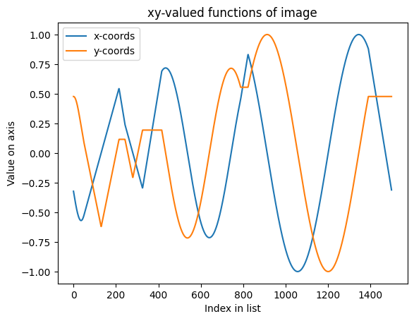
To draw our animation as a looping GIF, we are going to need to make sure our points start and end in the same spot. This can be done by looking at the functions that represent the $x$ or $y$ coordinate at a given time, and seeing if it is periodic.

We can visualize the functions that trace out the $x$ and $y$ coordinates below, where we see that both of our functions are periodic.

from matplotlib import pyplot as plt

# Plot the x and y coordinates
plt.plot(range(len(x_coords)), x_coords, label='x-coords')
plt.plot(range(len(y_coords)), y_coords, label='y-coords')

# Display the plot
plt.legend()
plt.xlabel("Index in list")
plt.ylabel('Value on axis')
plt.title('xy-valued functions of image')
plt.show()

Defining Epicycles

We are going to need a structure to hold the information for our spinning circles. The class below represents one of these circles, with the following attributes:

• Radius - The radius of the epicycle
• Theta - The angle in radians that the line in our epicycle has rotated so far
• Frequency - How quickly in Hertz the epicycle is rotating

# Create a class to represent the epicycloids
class Epicycloid:
    def __init__(self, radius:float, theta:float, frequency:int):
        self.radius = radius
        self.theta = theta
        self.frequency = frequency

Defining the Discrete Fourier Transform

As we have defined the DFT above, we will define it in code now. Recall that the DFT is defined as

\[X_k = \frac{1}{N} \sum_{n=0}^{N-1} x_n \left[ \cos{\left( \frac{2 \pi k n}{N}\right)} - i \sin{\left( \frac{2 \pi k n}{N}\right)}\right].\]

We can simplify this formula using Euler’s formula, which is defined as $e^{ix}=\cos (x) + i\sin (x)$. You may see where we can apply this to the DFT, where we can say

\[\begin{align*} X_k &= \frac{1}{N} \sum_{n=0}^{N-1} x_n \left[ \cos{\left( \frac{2 \pi k n}{N}\right)} - i \sin{\left( \frac{2 \pi k n}{N}\right)}\right]\\ &= \frac{1}{N} \sum_{n=0}^{N-1} x_n \cdot e^{-i\frac{2 \pi k n}{N}} \end{align*}\]

which is simpler to implement into our program. The implementaion is shown below, and makes use of the numpy package functions for lists to run the entire set of coordinates through the DFT at once.

import numpy as np
from typing import List

# Define the Discrete Fourier Transformation
def DFT(x: List[complex]):
    N = len(x)
    n = np.arange(N)
    k = n.reshape((N, 1))
    e = np.exp(-2j * np.pi * k * n / N)
    return np.dot(e, x)

Turning Coordinates into Epicycles

Now we can convert our coordinates into complex numbers, and run it through the DFT all at once.

# Convert x and y coordinates to a list of complex numbers
complex_coords = [complex(x, y) for x, y in zip(x_coords, y_coords)]

# Run our list of complex coordinates through the DFT
Xk = DFT(complex_coords)

Now that we have our phases and radii stored in $X_k$, we can turn the complex numbers into epicycles.

# Create an empty list to store Epicycloid objects
epicycloids_list = []

# Add our epicycloids
for k, X in enumerate(Xk):
    radius = abs(X)
    phase = float(np.angle(X))
    frequency = np.arange(len(Xk)).reshape((len(Xk), 1))[k]
    epicycloids_list.append(Epicycloid(radius, phase, frequency))

# Sort the list by radius in descending order
epicycloids_list.sort(key=lambda epicycloid: epicycloid.radius)
epicycloids_list.reverse()

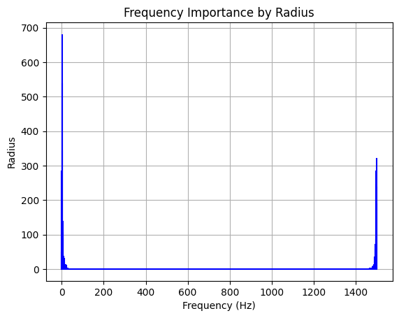
We can look at which frequencies store the most information by plotting the frequencies along the horizontal axis, and the radius along the vertical axis. the longer an epicycle’s radius is, the bigger difference it will make as it spins.

# Extract frequencies and radii from the epicycloids list
frequencies = []
radii = []

# Create our epicycloids
for e in epicycloids_list:
    frequencies.append(e.frequency)
    radii.append(e.radius)

# Plot the frequencies and radii
plt.stem(frequencies, radii, 'b', markerfmt=" ", basefmt="-b")
plt.xlabel('Frequency (Hz)')
plt.ylabel('Radius')
plt.title('Frequency Importance by Radius')
plt.grid(True)
plt.show()

Animating Epicycles

Now we can begin constructing our animation. First, we must choose how many of our epicycloids we wish to draw. The more we use, the more accurate it will be. i encourage you to change the value of this variable and see how the animation gets less accurate with less epicycles.

# How many of the epicycloids to use in our gif
NUM_EPICYCLOIDS = 50

# Remove extra epicycloids
epicycloids_list = epicycloids_list[:NUM_EPICYCLOIDS]

As we animate each epicycloid spinning end-to-end, we are going to need a function to both plot the epicycloid and calculate the end of its line.

from matplotlib.patches import Circle, FancyArrow
import math

def plot_epicycloid(t: float, epicycloid: Epicycloid, center_coords: List[float]):
    """
    Plot an epicycloid and return the graphical elements and new coordinates.

    Parameters
    ----------
    t : float
        The time parameter for animation.
    epicycloid : Epicycloid
        An instance of the Epicycloid class.
    center_coords : list of float
        The x and y coordinates of the center of the epicycloid.

    Returns
    -------
    Tuple containing:
        - Tuple of matplotlib.patches.Circle and matplotlib.patches.FancyArrow
        - Tuple of new x and y coordinates as floats
    """
    # Plot circle
    circle = Circle(center_coords, radius=epicycloid.radius, color='black', fill=False, alpha=0.25)

    # Calculate ending point of the line
    x, y = center_coords
    dx = epicycloid.radius * math.cos(epicycloid.theta + t * epicycloid.frequency)
    dy = epicycloid.radius * math.sin(epicycloid.theta + t * epicycloid.frequency)

    # Plot line
    line = FancyArrow(x, y, dx, dy, color='black')

    # Return the circle and line, and the new coordinates
    end_of_line_coords = (x + dx, y + dy)
    return (circle, line), end_of_line_coords

We are using FuncAnimation from matplotlib.animation to create our animation. This means that we need a function to be called every frame to create our new plot.

from matplotlib.patches import PathPatch
from matplotlib.path import Path

def animate(frame: int, epicycloids: List[Epicycloid]) -> Tuple[List,]:
    """
    This function is for the FuncAnimation to call when it wants to draw a frame.

    Parameters
    ----------
    frame : int
        The current frame number in the animation.
    epicycloids : list of Epicycloid
        A list of Epicycloid objects to be animated.

    Returns
    -------
    tuple
        A tuple containing a list of artists to be animated.
    """

    # Scale our frame value to [0, 2pi]
    t = (frame / FRAMES) * 2 * 3.14159265

    # Clear our graph and update boundaries and title
    ax.clear()
    ax.set_xbound(-1600, 1600)
    ax.set_ybound(-1600, 1600)
    plt.title(f'{NUM_EPICYCLOIDS} Epicycloids')

    # Keep track of every object that needs to be plotted
    iterable_of_artists = []

    # Define the origin as the starting point
    x, y = 0, 0

    # Calculate where each epicycloid should be at this frame time
    for epicycloid in epicycloids:

        # Get current epicycloid plot data and next coordinates
        artists, next_coords = plot_epicycloid(t, epicycloid, [x, y])
        x, y = next_coords

        # Plot the epicycle and add the new plot data to our list of artists
        for artist in artists:
            ax.add_artist(artist)
            iterable_of_artists.append(artist)

    # Add the last (x,y) coordinate to our plot to be traced
    traced_line.append((x, y))
    path_patch = PathPatch(Path(traced_line), color='blue', fill=False)
    ax.add_artist(path_patch)
    iterable_of_artists.append(path_patch)

    return iterable_of_artists,

Now we can create and save our animation!

%%capture
# ^ This prevents useless outputs of random animation frames

from matplotlib.animation import FuncAnimation

# Define constants
FRAMES = 500 # Be careful of making this too low or high. Usually 500 works well
INTERVAL = 50 # Delay between frames in milliseconds

# Create our canvas
fig, ax = plt.subplots()

# Keep track of the points being traced
traced_line = []

# Create a list of frame values to evaluate
frames_list = np.arange(0, FRAMES)

# Create and save the animation (this may take a long time depending on FRAMES)
animation = FuncAnimation(fig, func=animate, frames=frames_list, interval=INTERVAL, fargs=[epicycloids_list])
animation.save(filename=f"gvsu-logo-dft-{NUM_EPICYCLOIDS}.gif", writer="pillow")

If you are using an intereactive Python environment such as Google Colab, we can display the gif right in our editor!

from IPython.display import Image

# View the gif in Google Colab
Image(open(f"gvsu-logo-dft-{NUM_EPICYCLOIDS}.gif",'rb').read())

Results

How exciting! We have succesfully created our own epicycloid animation using the Discrete Fourier Transformation!

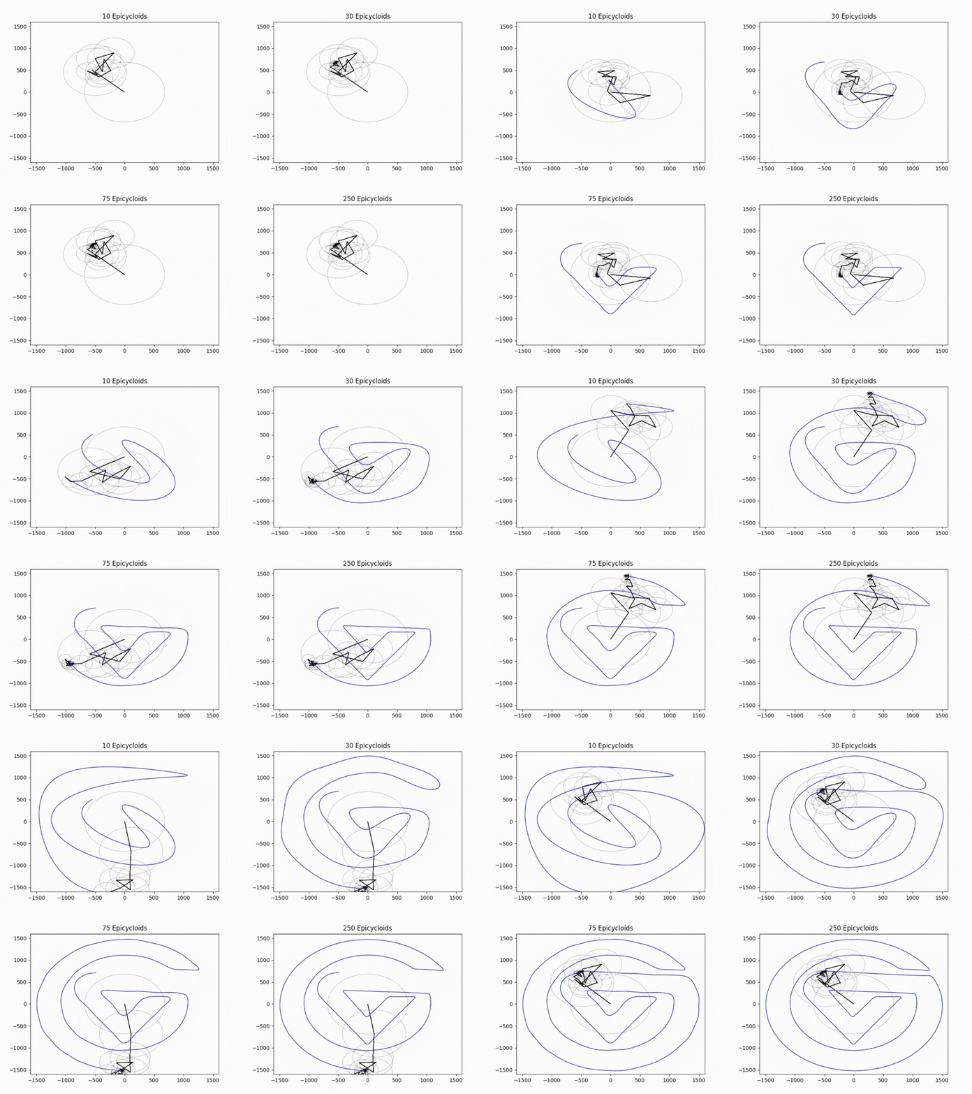
I find it interesting that reducing the number of epicyloids used in the animation reduces the quality of our drawing, almost like an incredibly complicated form of compression. This is shown below in the gifs using 10, 30, 75, and 250 epicycloids.

In the future, I would like to make this applicable for any traceable shape. This means I would have to find a way to convert .SVG files reliably with python, and possibly auto-adjust any variables specific to my image.

Additional Resources

In my research, I found an incredibly helpful paper by Juan Carlos Ponce Camuzano titled Tracing closed curves with epicycles: A fun application of the Discrete Fourier Transform. This paper was a massive help throughout this project, and I encourage you to read it to fill the gaps on what I couldn’t fit into this post.

YouTuber 3Blue1Brown has an excellent video titled But what is a Fourier series? From heat flow to drawing with circles which introduced me to the idea of drawing with the DFT. He has created several videos on the DFT, which I reccomend watching as well.

Additionally, YouTuber The Coding Train has a video titled Coding Challenge #130.1: Drawing with Fourier Transform and Epicycles which goes into the implementation of these animations using JavaScript. While I implemented mine in Python, the broader ideas he used were very helpful to me.